Houston Updates

Houston’s Outlook Reshaped by COVID-19 and the Oil Collapse: Perspectives on the Economy from the Early Pandemic Data

June 28, 2020

This article is a second update of what has become an ongoing report on the outlook for the Houston economy due to COVID-19.¹ The first report on the impacts of COVID-19 and a major oil downturn was published on March 22, but promptly updated on April 8 to account for the switch in perspective on COVID-19's economic impacts from an illness and labor-shortage driven event to one given new direction by public health stay-home mandates that closed large parts of the U.S. economy.

Also, it has become clear that the winner of the oil war had been declared, and it was neither Saudis nor Russians — but COVID-19. Deep cuts in global oil demand from stay-home orders and business closings around the world have meant a long period of low oil prices ahead, with no need to look elsewhere for the cause. Thousands more local oil jobs are now at risk.

This reworking of the outlook is also the result of new employment data available through May, the first meaningful numbers received on the effects of the virus and the economic damage reported so far. The data show huge losses, but also the first clear signs that Texas and Houston have bottomed out and that we are making economic progress as the economy reopens. The following section summarizes results.

This report remains highly speculative. This is partly because we are early in the downturn and the economic data remain limited, but primarily because the COVID-19 virus remains largely uncharacterized. There is no firm data on the rate of infection or mortality, whether reinfection is possible, or how long until there is effective treatment or a vaccine. The economics, including such basic facts as the potential length and depth of the downturn, remain heavily dependent on unknown basic facts about the virus.

Today’s Perspective on This Pandemic: A Summary

As we work our way through the current public health and economic crisis in Houston, the outlook continues to evolve rapidly. Past pandemics have seen public health officials implement a variety of protective measures such as quarantines, school and theater closings, and limiting crowd size, but the COVID-19 intervention in the economy through stay-home orders and widespread business closings has been unprecedented.

The immediate loss of 349,700 jobs in Houston in March and April is largely the result of stay-at-home orders by local public health officials plus reactive social distancing by the public. These stay-home orders were deemed necessary to ration hospital capacity and other essential services and to save lives, but they also radically changed the near-term economic outlook and our understanding of how economic events will unfold in the face of a serious pandemic.

Past pandemics have followed a different schedule: the virus spreads, there is reactive social distancing by the public that leaves stores and restaurants half empty, illness becomes widespread among workers, labor shortages force shift reductions and plant closings, economic uncertainty slows business and consumer spending, and different cities at different times close schools, limit crowds, and issues various public orders. The result was an economic shock, but one that unfolded over a period of weeks and months and not a few days.

The unprecedented widespread stay-home orders and closing of nonessential businesses pulled all of this forward in time — all the adverse effects came at once — creating a much larger economic shock than ever seen previously, and then unprecedented community-wide quarantine and business closings came on top of this.

There is trade-off here. As difficult as the stay-home orders are for businesses struggling to survive, if this enforced social distancing failed, we would still have seen substantial economic losses as well as many more deaths. A pandemic that did not employ pre-emptive business closings would none-the-less see heavy job losses that would just occur later in the infection cycle, as big swaths of the labor force were lost to illness and family caretaking. Reactive social distancing still would have left many restaurants and retail stores half empty.

The combination of stay-home orders and nonessential closings, plus the large and unexpected shock it generated, probably created more economic damage than would have occurred otherwise. However, as fast as the public health orders put people out of work in March and April, the Treasury Department was replacing their lost income. If we saw the largest decline in employment in history, it was met with the largest-ever increase in personal income as fiscal policy made up the losses in wages, salaries, and proprietors income. Even as employment fell by over 20 million, trillions in stimulus payments allowed personal income to rise measured from March to May and to generate large personal savings by consumers.

Where does the Houston economy go now? We divide the likely post-COVID-19 economy into two parts. First, there is the effect of the disease on the broad U.S. economy as the virus progresses and brings a recession that is likely to last twelve months or more. Based on a growing number of studies of the relatively modest economic impact of a severe Spanish Flu pandemic, a bottom-up study by the Congressional Budget Office on the effects of past pandemics, and early data on the current economic reopening, we think Houston will share a moderate U.S. recession that unfolds over several quarters. It is fiscal spending that offsets losses to employment and provides balance to our outlook, and it is unlikely that the resulting recession will be nearly as bad as projected by many analysts who focus too narrowly on job loss alone.

Houston will share the national downturn as it loses sales to the rest of the state, country, and world. If we focus on Houston’s economic base — those industries that drive economic expansion and contraction — the early March to May data indicate a local recession that so-far ranks as typical of the average local downturn we have experienced since 1990. The current Houston Purchasing Managers’ Index is now telling a similar story.

The second part of Houston’s near-term economic situation is the mandatory stay-home orders and business closings, combined with the normal reactive social distancing by the public. These local decisions depend narrowly on the progress of the virus and the reaction of public health officials, and it is simply unpredictable. However, a reasonable illustrative example can show how social distancing explains the large and frightening month-to-month changes we see in local employment, and how a successful economic reopening quickly swings the job figures from large negatives to equally-large positives.

Adding to the angst for Houston is the recent collapse in demand for oil as the Chinese, U.S., and European economies ground to a halt. Current low oil prices again raise the likelihood of Houston seeing a significant economic setback, although signs of stability are returning to oil markets faster than expected. Unfortunately, a return to fundamentals does not mean the fundamentals are particularly good.

After the illness subsides, public orders and economic disruptions end, and social distancing is no longer needed, where will we find the Houston economy? Assume the virus runs its course in 2020, and that the stimulus package is an effective economic bridge, by early 2021 the U.S. and Houston will begin a year of recovery from moderate recession. That recession would mean the loss of 72,800 jobs measured from 2020Q1 through 2021Q1, with recovery of employment complete by 2022Q2. As recovery unfolds and turns into expansion, we will see strong growth in 2022 and 2023 followed by a return to trend growth.

COVID-19 and Lessons from Past Pandemics

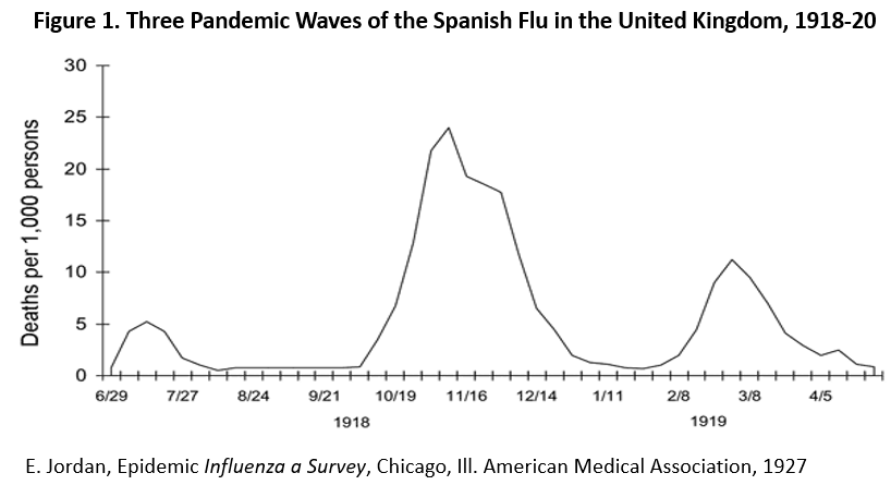
Past viral epidemics and pandemics such as influenza began with a local outbreak of the disease that spreads to other regions, the number of cases reported then grows rapidly, and the virus may remain widespread from three to six months. The number of infections and deaths peak and decline after much of the population develops a natural immunity, with a smaller second wave possible one or two months later. See Figure 1. The number and timing of these waves of Spanish Flu were very similar to Great Britain and the U.S.

Influenza and other viruses bring a sudden and urgent need for medical services as a large share of the population finds itself infected. Figure 2 shows the case infection rate for four pandemics that have occurred since 1918. For the Asian, Hong Kong, and Swine Flus, we see 7-28 percent of the population infected, and case fatality rates that means 0.2 to 0.3 percent of those infected will die.

The Spanish Flu stands out with its 33 percent infection rate and 2-3 percent fatality rate. Influenza has typically struck hardest among the youngest and oldest age groups, but the Spanish flu also hit quite hard among prime-age groups. In 1918, 272,500 males died of the flu, with 49% of deaths in the 18-40 age group, and only 18% among those under age 5 and 13% over 50.² This made economic losses to the Spanish flu much worse with the heavy losses of prime-aged and single-earner workers.

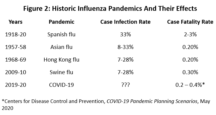
The Centers for Disease Control and Prevention (CDC) released a May planning document that places the overall case fatality rate for COVID-19 at 0.2 to 0.4 percent, although it hits older Americans above age 65 much harder with rates estimated from 0.6 to 3.2 percent. For those under 50, the case fatality rate is .0005 or one in 2000.³ The range of variation in the estimates depends on differing assumptions about virus transmissibility, disease severity, rate of transmission prior to symptoms, and the percentage of cases that never show symptoms.

Are there lessons from the past for the U.S. economy? Perhaps for the 1918-19 Spanish Flu, but is unclear if there is an adverse economic link between the Asian, Hong Kong, or Swine flu pandemics. The Hong Kong Flu came well in advance of the 1968-69 recession and no link has been established to the recession that followed, and the Swine Flu began to spread after the trough of the Great Recession in 2009. The 1957-58 Asian flu coincided closely with a mild recession, although the downturn is typically blamed on tight monetary policy and budget tightening. However, it is also sometimes cited as a potential model for the macroeconomic consequences of a moderate pandemic: a significant slowdown in GDP growth, perhaps falling to near zero, but probably not sufficient to cause recession.⁴

The Spanish Flu stands as the model for a severe pandemic, killing 675,000 Americans and 40 million worldwide. It was relatively short-lived but while active it killed at a faster rate than the Black Death of the 1300’s. Economist Robert Barro ranks the three greatest modern macroeconomic disasters as World War II, the Great Depression, and World War I, but gives the Spanish Flu epidemic a likely fourth place.⁵

Moving from flu-driven mortality rates to the economic consequences of the 1918-19 pandemic has proved challenging because of other extraordinary events underway at the time: the U.S. industrial build-up to WWI (1914-17), U.S. entry into WWI (1917-18), a mild recession that coincided with the Spanish Flu (1917-18), and the second-worst recession in U.S. history driven by post-war demobilization (1920-21). Economists anxious to tell a story about the virus often have been to slow to recognize the need to control for WWI mortality or to recognize the limits of widely available annual data in sorting these overlapping dates.⁶

A key question has been whether there was only the mild 1918-19 recession that defined the macroeconomic consequences of the Spanish Flu, or whether the flu’s effects spilled into the much more severe recession of 1920-21. The two recessions still stand on the definitive list of recessions published by the National Bureau of Economic Research, and their positions is based on work originally done by Wesley Mitchell and Arthur Burns in 1946.⁷ In response to recent challenges as to whether there was one recession or two, Velde revisited the issue with the Spanish flu explicitly in mind.⁸ He uses much of the same high-frequency data used by Mitchell and Burns (employment, retail sales, industrial production, bank clearings, etc.), confirms the original story regarding the length and depth of the recession, and reinforces it substantially from other sources. He also finds that the mortality rates from the Spanish flu were statistically important in industrial activity, less so in employment, and mixed or not significant in most other series. He concludes “that the pandemic coincided with, and very likely contributed to, a mild recession from which the economy rebounded quickly.”

The most recent entry into studies of the macroeconomic effects of the Spanish flu has been the work of Barro, Ursúa, and Weng.⁹ They use a panel of 42 countries and annual data on GDP and personal consumption from 1901 to 1929 from each country to explicitly account for and separate the effects of WWI and Spanish Flu mortalities.

• They find the average loss to the 1918-19 pandemic across 42 countries was a decline in GDP of 6.2 percent; for WWI, the mortality rate forced a decline in GDP of 8.4 percent. Hence, Barro’s claim that the Spanish Flu probably ranks fourth among macroeconomic disasters after WWI.
• However, the U.S. death rate to the Spanish Flu at 1.5 percent was small compared to global deaths, resulting in flu-related losses to U.S. GDP of only 1.5 percent. The mortality rate from WWI cost the U.S. 2.9 percent of GDP.
• The authors claim the data quite clearly point to two recessions — 1918 and 1920-21 — based on both the timing and the size of the downturns. The Spanish Flu is again found to coincide with a mild and short U.S. recession that would be difficult to stretch into a longer and more serious event lasting until 1920 or beyond.

In 2006, the Congressional Budget Office was asked to prepare a report in response to concerns about the potential macroeconomic effects of a virus-driven pandemic. The concern at the time was the Avian Flu, but their results would apply to any potential pandemic. This study contrasts to the statistical analyses of pandemics discussed above, instead breaking the effects of a future pandemic into losses to supply and demand. Interruptions to supply are the consequence of large numbers of worker illness, labor shortages, shift reductions, plant closings, and material shortages due to supply-chain disruptions. Demand is reduced by reactive social distancing driven by fear of the virus that would reduce activity in sectors such as travel, transportation, hospitality, personal services, and retail.

Even in 1918-19 there would be public health measures imposed such as quarantine, school and theater closings, and crowd limits. Uncertainty about the health and economic consequences of a spreading disease would further cut business and consumer spending. Widespread business closures were not envisioned in this 2006 study. Estimates of losses were made on a bottom-up basis and were estimated industry by industry. There are three scenarios.

• The first scenario is a base case with minimal consequences beyond a typical seasonal outbreak of influenza. From a macroeconomic perspective, trend growth would continue.
• The second is a mild pandemic that assumes 25 percent of the population (82.5 million people today) would become infected and a 0.16 percent case fatality rates means 135,000 Americans would die. The CBO estimates this would reduce GDP by 1.0 percent or more compared to what would have happened without the pandemic, but it might not slow the economy enough to cause recession.
• The severe case is based on the Spanish Flu of 1918-19, with a case infection rate of 30 percent (99 million will fall ill) and the case mortality rate of 2.3 percent means 2.3 million U.S. deaths. The macroeconomic results of the virus are a four quarter decline of 0.6 percent per quarter, or 2.5 percent over the following year. This would be a recession typical of recessions seen in the United States since 1948. Once more, a moderate recession is linked to a severe pandemic.

This four-quarter decline of 2.5 percent would contrast with a fall of 4.0 percent over six quarters of the Great Recession, for example, with GDP falling at annual rates of 8.4 percent in 2008Q4. More striking is the current outlook from the Survey of Professional Forecasters that sees a decline of 32.2 percent in GDP in the current quarter and 5.6 percent for the year.¹⁰

That said, we will later argue at length in this report that there is value in considering how the 1918-19 epidemic generated only moderate cyclical impacts. Much of the short-run damage presented by the Survey is the effect of quarantine of all nonessential workers and enforced business closing, and a good part of the damage is lost income that is covered by $3 trillion in fiscal funds and more in monetary stimulus. If federal policy works as planned, a moderate underlying recession reflects what is left after stay-home orders, enforced closings, and federal policy are finished.

Figure 3 summarizes how the CBO scenarios might look if stated in terms of U.S. payroll employment. I use employment because it is the key variable for our Houston forecast. The figure shows a base forecast with continued trend growth. There is a mild U.S. recession over four quarters with a 1.5 percent (or 2.3 million jobs) decline in payrolls, followed by four quarters of recovery or a return to the prior peak.¹¹ The severe recession is a four-quarter decline in employment (4.6 million jobs) followed by five quarters of recovery. The hypothetical recessions both begin in 2020Q1, end 2021Q1, and find employment recovery complete by after four quarters for the mild recession and five for the severe.

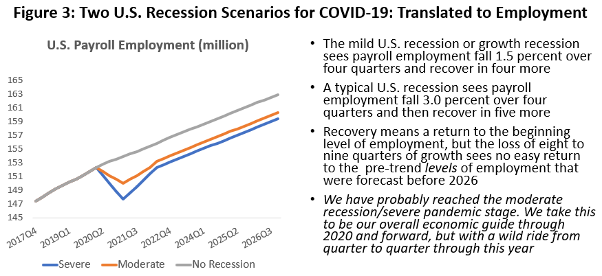
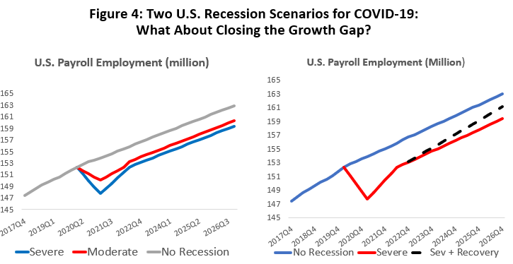
Figure 4 shows the same three scenarios as Figure 3 on the left, but the chart on the right focuses on the severe downturn. Large external shocks like a pandemic generate losses that can be permanent in the sense of never returning to the prior growth path. The red line in Figure 4 shows the loss to recession and a return to the prior growth rates that begins only after recession has ended and recovery is complete. The difference between the blue line and the red line then become the permanent losses. It is possible, however, that the past losses can be made up. For example, the broken black line represents a post-pandemic acceleration in growth that reflects partial recovery from macroeconomic disaster, with half the losses made up by 2026.

The study of the effects of flu mortality on economic growth in the 1918-19 pandemic by Barro, Ursúa, and Weng tested statistically to see if the losses were permanent or temporary, but found the results inconclusive — flu-related losses in GDP could be permanent, partial, or completely recovered. For WWI, however, the authors found that about half the losses were made up in later years, a result Barro has found typical of other macroeconomic disasters.

The CBO asked the same question about the interpretation of their hypothetical pandemics. While their severe case would have meant the death of a million workers, they also found the prospects for any recovery from the shock indeterminate. Like Barro, et al., losses could be permanent, partial, or complete. In their analysis, the capital-labor ratio could rise with the heavy loss of workers and perhaps result in a long period of declining investment. Alternatively, the loss of so many workers could trigger extensive new training and education programs that would result in rising per capita income.

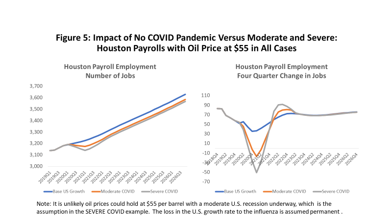
Figure 5 illustrates how Houston is affected by these hypothetical recessions. It shows the performance of Houston’s payroll jobs through the COVID-19 downturn and assuming that the price of oil is fixed at $55 in all three cases. We will add oil to the simulations later, but this chart tells us a familiar story about how Houston is typically less affected by U.S. economic downturns than the rest of the country.

The mild downturn of 1.5 percent employment in the U.S. sees Houston’s job growth shrink slightly through 2020q1, with a moderate loss of 17,400. The severe COVD-19 case would imply the loss of 54,500 jobs. This compares to 49,000 net new jobs that we had forecast for this year as recently as January. The more serious U.S. recession translates into a Houston downturn that is half as deep as the rest of the country in percentage terms, but it still results in meaningful recession. Adding the current oil losses later worsens the outcomes for Houston.

This Is Not Yesterday’s Pandemic Response

Reconciling the hypothetical recession and the resulting loss of only 54,500 local jobs contrasts substantially with 349,700 jobs lost in Houston in March and April. It leaves a very large gap to fill. Doing so requires a substantial discussion of the stay-home orders and closings of nonessential business, an experiment never previously tried on a significant scale. It also requires a discussion of the massive investment made by the Treasury and Federal Reserve in substantially offsetting the economic effects of these job losses.

Many would like to find the debate on the use of public orders versus the economy fitting neatly at one polar extreme or the other, with an inherently positive or negative outcome for whichever view they hold. But like most of economics there are tradeoffs at work, and the public orders come with a difficult weighing of plusses and minuses regarding economic outcomes.

The use of stay-home orders and the widespread closing of nonessential businesses have added to the arsenal of tools available to public health officials to slow the spread of a virus and to prevent capacity from being exceeded by hospitals and other essential services. However, these orders have also brought unprecedented intervention in the economy , and they have changed the course and economic consequences of the virus. They have added greatly to the extraordinary job losses seen in March and April, although — as we will see — many of those losses would have occurred in the absence of the orders, just at a later point in the course of the pandemic.

The 1918-19 Spanish Flu in the United States provided many examples of public health policy measures that used enforced social distancing to slow the spread of the virus. Called nonpharmaceutical interventions (NPIs), a 2007 study by Markle, et al. looked at the variation in mortality across 43 cities that employed these tools in 1918-19.¹² The authors considered three major groupings of NPIs: school closings, cancellation of public gatherings, and isolation/quarantine. The NPIs typically worked best as a combination, with school closings and cancelled public gatherings making up the best pair, for example. The NPIs were found to allow cities to reach peak mortality more slowly, to lower peak mortality, and to lower overall mortality.

Bootsma and Ferguson similarly find a profound effect of NPIs on 1918-19 mortality based on a statistical analysis of 16 U.S. cities and a mathematical extension that used parameters from those 16 to construct an epidemiological model of a broader group of 43 cities. ¹³ The model results combined reactive social distancing with the public health NPIs to estimate the interaction between them. They found, for example, that the second peak in many cities could be interpreted as the initial NPIs having been too strict and leaving a large segment of the population unprotected when orders were lifted. Orders typically had been lifted within four to six weeks. The theoretical reductions in peak mortality could be as high as 40 percent, but practical obstacles to real-time implementation allowed only four cities to reach 30 percent.

The primary contribution of Hatchett, Mecher, and Lipsitch was to expand this list of 1918-19 NPIs to 19 measures in 17 cities.¹⁴ The most widely used NPIs employed by 10 or more cities were making influenza a notifiable disease, isolation and quarantine, various mandated public closings, private funerals, and bans on public gatherings. Implemented in five or fewer cities were emergency declarations, mask ordinances, protective sequestration of children, limiting crowding in public spaces, and community=wide business closings. This last measure was implemented in only one city during the Spanish Flu. Their study finds peak mortality was reduced by these measures by as much as 50 percent, but the return of a second peak meant the cumulative mortality fell to 20 percent or less and could be measured only with less statistical significance.

The ingredients of a 1918-19-style pandemic, or the 2006 pandemic envisioned by the CBO, would occur in the following order: (1) immediate reactive social distancing and fewer customers in bars, restaurants, retail stores, barber shops, etc.; (2) as the disease spreads, hundreds of thousands of workers across many industries fall ill resulting in shift losses, plants being shut down, supply-chain disruptions, etc.; (3) economic uncertainly spreads along with the virus and consumer and business spending fall; (4) herd immunity finally protects a meaningful part of the community and the virus slowly recedes after a first or second wave of infection; (5) NPIs were widely used in past outbreaks but implemented by different cities at different times and different points in the pandemic.

The recent use of widespread stay-home orders and nonessential-business closings bunches all of the adverse events together just as the virus emerges — the shock of the virus, reactive social distancing, a huge economic shock and associated uncertainty, and immediate and very large employment losses. Many of the job losses would have occurred later anyway in the course of the epidemic and mortality rates are reduced by the orders, but the stay-home policy caused an immediate economic shock much greater than anything seen in the past. The March/April payroll job losses for Houston, for example, totaled 350,000 in reaction to the virus and the public health orders, compared to the 211,000 jobs lost to Houston’s massive oil downturn that lasted from 1982 to 1987.

Figure 6 considers how the virus might have played out in Houston without the new public orders and using the CBO’s definition of a severe pandemic. With seven million Houstonians and four million payroll and self-employed workers, a first and second wave, and two weeks of absence per worker that falls ill, we see several weeks at the peak of the pandemic with job losses that would see 160,000 to 240,000 out of work.¹⁵

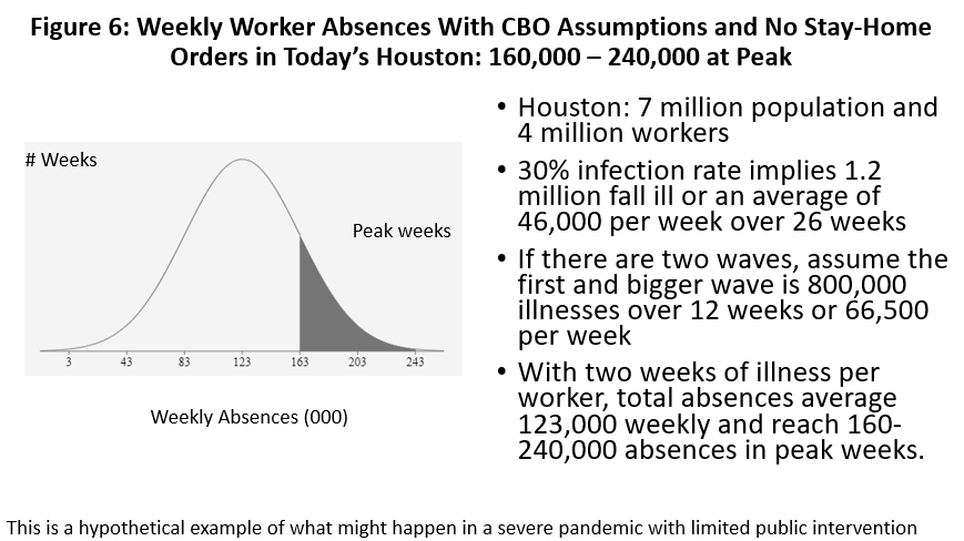
There is clearly a trade-off between the early-pandemic/enforced job losses from public health orders and later job losses as tens of thousands are stricken by the virus. I am not going to even try to compare the number of job losses between these two different situations, especially with the data we have at hand, but job losses are likely made worse by stay-home orders and the huge economic shock that came with this first-ever experiment.¹⁶

On the other hand, a 2.5 percent mortality rate under the CBO scenario would mean the death of 30,000 Houstonians. Even under the current CDC’s May planning assumptions of a 0.4 percent mortality rate, 4,800 would die. On this score, the June 10 morbidity and mortality figures for Harris County tilt in favor of the effectiveness stay-home orders with only 12,200 confirmed case of COVID-19 and 231 confirmed deaths.¹⁷

Where We Stand Now

The data in the previous section described an on-going hypothetical but run-of-the-mill recession involving the loss of 4.5 million U.S. jobs and 54,000 layoffs in Houston. But just in March and April we saw 22.1 million U.S. payroll jobs disappear, with 350,000 of them in Houston. It is by only looking at detail buried in the recent data — where the losses are coming from and their importance in driving the economy — that we can begin to reconcile some of the accounting used in two very different versions of a similar story. We will see that key elements of Houston’s current employment picture are still pointing to moderate recession. And the trillions of dollars in emergency fiscal and monetary policy play an important role in providing economic balance to frightening job losses by replacing much of the income of those who lost their jobs.

The most current economic data since the pandemic began are weekly figures on initial and continued unemployment compensation claims that are available through mid-June for the U.S. and Texas. The left side of Figure 7 shows the continuing effect of what became a rolling avalanche of claims that peaked on March 28 in the U.S. at 6.9 million, and then peaked a week later in Texas at 315,000. The timing and extent of the job loss driving these claims suggests a common large factor at work, and the shock of public health orders is the likely culprit.

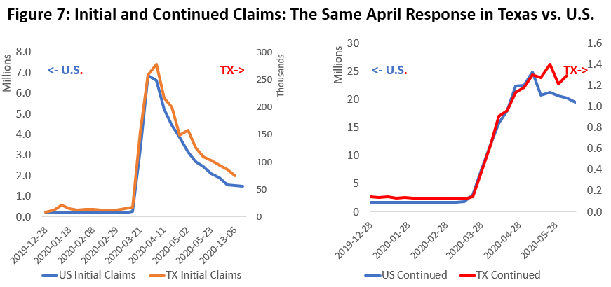
After peaking, the initial claims have fallen back to much lower levels, but the right side of Figure 7 shows that continued claims (total initial claims less claims terminated by ineligibility or by claimants finding work) remain above 20 million in the U.S. and 1.2 million in Texas. U.S. claims peaked in early May, followed by Texas two weeks later, although Texas’ claims struggle to make progress.

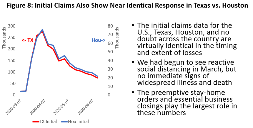
The initial claims on the left side of Figure 8 compare Houston to statewide results, and we see the same April surge and timing of initial claims. We do not have continued claims data for Houston, but there is little reason to think it would look much different than Texas.

The payroll employment data for March and April tell us which sectors drove most of the 22.1 million U.S. job losses and the 350,000 lost in Houston, as well as the partial recovery that came in May as the economy began a measured reopening. The list of industries in Figure 9 makes up almost 70 percent of the March/April losses when the stay-home orders were imposed and nonessential businesses were closed. They are the sectors most sensitive to enforced or reactive social distancing — accommodation, entertainment, food service, retail, etc. In May we saw the Houston economy bottom out, with a net return of 65,800 jobs, or 20.4 percent of the previous losses. The U.S. saw 2.5 million jobs come back or 11.4 percent of the prior decline.

Job recoveries in May, like earlier losses, came mostly in distancing-sensitive sectors led by health care, food service, and retail. Over the next few months, if we avoid a second peak and public health mandates remain lifted, these sectors should continue to show mostly job loss to reactive distancing. But if the virus cooperates, we expect even reactive losses to slowly decline through the year as businesses learn to work around the virus and the public becomes less wary.

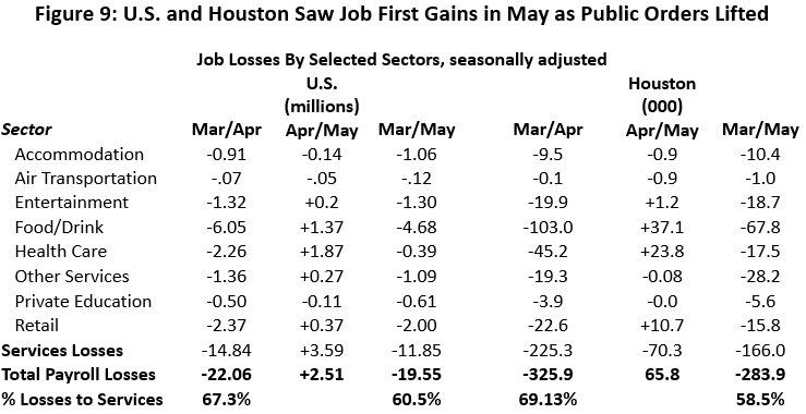
Figure 10 puts these losses in distancing-sensitive sectors into perspective relative to other losses throughout the economy. This data runs through May and includes the early reopening phase and partial job recovery. The yellow box contains the same distancing-sensitive sectors as the previous chart. We see the additional losses to upstream oil (18,000), professional and business services (24,700), construction (23,700), finance (3,100), other manufacturing (9,300), and other sectors (29,400). Upstream oil directly accounts for 6.6 percent of job losses. Many of these sectors see losses triggered by consumers and businesses pulling back due to the nationwide recession. This pullback comes in sectors like employment services, construction, and professional and technical services.

At the bottom of Figure 10, the green box describes an accounting of recent job losses in Houston’s economic base, divided into losses driven by oil and by other sectors. The economic base concept is a relatively naïve but useful concept in regional economics, helpful for both descriptive and analytical purposes. We use it here to describe a likely on-going moderate recession in Houston due to the pandemic, a description that does not rely on any appeal to a CBO-like national recession or even to a virus.

The economic base is the group of industries and firms that drive the local economy. To drive growth, they must be able to sell their goods and services outside the region or to other parts of the state, nation, or world. They make us richer by bringing new income into the community. Goods sectors like agriculture, mining, and manufacturing are typically basic or primary, but any company counts as basic that sells local production outside the region, e.g., Sysco, AIG, Waste Management, or Men’s Wearhouse.¹⁸

Non-basic or secondary activities are inherently local, selling goods and services into the community. They do not generate new income from outside the area, and we do not get rich taking in each other’s laundry. Our selected services that are sensitive to social distancing in Figure 9 are almost all non-basic or secondary, with the exception of air travel and some parts of health care like foreign patients, research, and education. Without belittling any job or line of business, these industries are not the drivers of local expansion or recession. In fact, they are typically the most stable part of the economy, in contrast to the highly cyclical basic industries.

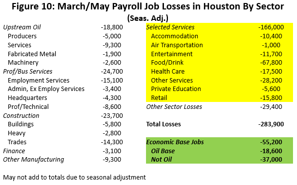
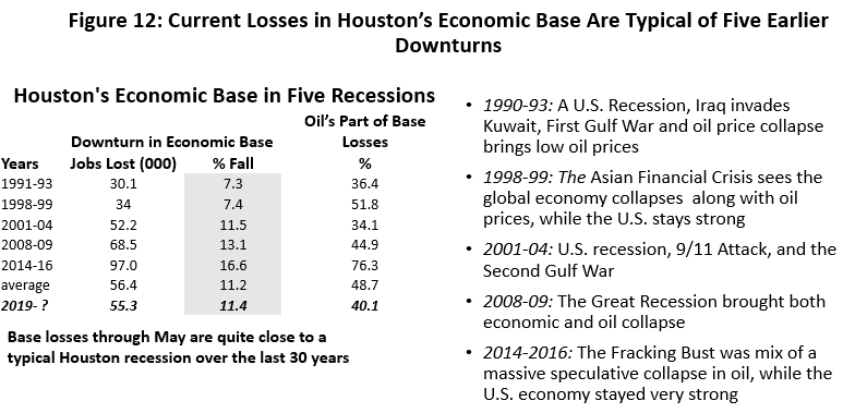
Figure 11 shows Houston’s economic base measured in thousands of jobs and divided into oil-related and other sectors. It shows five downturns in the local economic base since 1990: the 1990-91 U.S. recession and the First Gulf War; the 1998-99 Asian Financial Crisis; the 2000-2004 U.S. Tech Bust and Second Gulf War; the Great Recession and an associated oil downturn; and the 2014-16 Fracking Bust. Each of these events led to a local recession or growth recession.

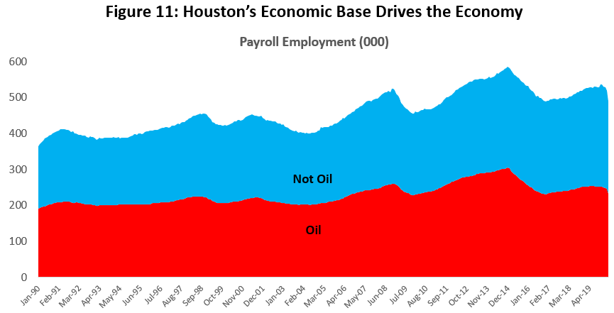
Figure 12 shows the number of basic jobs lost to each downturn, the percentage of base jobs lost, and the percentage share of losses that can be attributed to oil. Basic losses by event range from 30,100 jobs or 7.3 percent of the base in the relatively mild 1990-1993 downturn to 97,000 and 16.6 percent in the Fracking Bust. So far, the March/April/May losses are 55,300 or 11.4 percent, and this stands in the middle of the pack compared to Houston’s modern business-cycle history. So far, the current local recession is typical of downturns over the last 30 years. This moderate recession is not based on any CBO-style estimate of the local consequences of an assumed national downturn — it is just what we see in the Houston data right now.

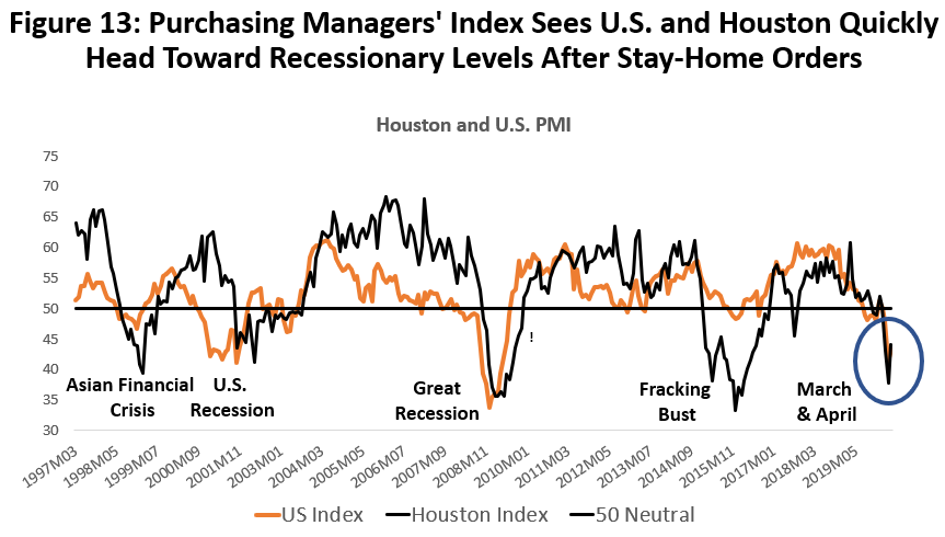
We can turn to Houston Purchasing Managers’ Index (PMI) as another data source that tells us a similar story of moderate recession, in this case based on monthly survey results. Figure 13 shows the history of the local PMI since 1997 compared to the U.S. manufacturing PMI. If the value of either index is greater than 50 it indicates economic expansion, and less than fifty means contraction. The local index clearly reflects and reproduces the same history of recent downturns as the earlier economic base calculations.¹⁹

Beginning in February, the seasonally adjusted index values for Houston have been 50.3, 43.2, 37.8, and 44.0; for the U.S. they have been marginally better at 50.0, 47.9,41.4, and 43.3. For Houston and the U.S. these indexes are indicating a contraction that falls well into recessionary levels, but they are not the worst downturns ever recorded. The U.S. saw the index fall to 33.7 in the Great Recession and 41.1 in the relatively mild 2000-2001 recession. Houston fell to 33.3 in the Fracking Bust, 35.7 in the Great Recession, and the 39.4 recorded in the Asian Financial Crisis almost matched the recent low. This again suggests that while a major shock is underway, it is not unexplored territory.

Filling the Gap? Trillions of Dollars in Stimulus

As we go back and forth between data pointing to millions of jobs lost to an abrupt economic shock and other data pointing to a recession that we have seen a couple of times before in recent years, the missing gap is trillions of dollars in federal monetary and fiscal stimulus. On the one hand, we have the public health authorities temporarily (and with well-meant intentions) destroying millions of jobs in March and April to reduce COVID-19 mortality rates, and on the other is the Treasury Department generating the largest increase in personal income in history to offset job loss by replacing the wages and salaries of the unemployed. As shocking as the job losses are, it is the net effect that determines the depth of this recession.

Congress and the Federal Reserve have met the challenge of economic collapse with an all-out effort to replace income lost to the pandemic and to make credit cheap and widely available. The Treasury stimulus package now totals $2.9 trillion and is summarized in Figure 14. The stimulus often has been described as a bridge from the pre-COVID to a post-COVID economy. On one side is the massive job loss from reactive and enforced social distancing and on the other side is the equally massive income replacement for those who lost jobs. The $1.3 trillion in stimulus aimed at protecting jobs, making direct payments to individuals, or supplementing unemployment insurance is enough to pay $38,900 to 33.4 million working Americans for a year, an amount equal to 80 percent of the average annual U.S. wage or salary earned in 2019.²⁰ The size and length of the stimulus bridge appears fully adequate for the early stages of the pandemic, and Congress seems willing to provide more stimulus if it proves necessary. The other question is whether the money will prove effective in reaching the households and businesses that most need it.

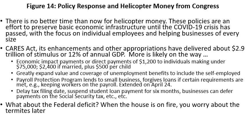
Figure 15 shows the immediate economic consequences of the stimulus spending in March, April, and May. Personal income rose $168.2 billion in April, the largest increase in history. This was the result of a monthly jump in government transfers of $252.3 billion, more than offsetting a loss of $70.0 billion in wages, salaries and proprietors income as employment plummeted. The increase in government transfers was led by the one-time economic impact payments made through the IRS, plus the enhanced unemployment compensation. This increase in transfers was four times the April loss in total compensation.

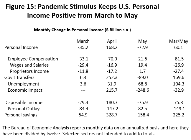
Further, while disposable income rose by $180.7 billion in April, personal outlays were slowed by economic uncertainty and discouraged by stay-home orders and closings of nonessential businesses. The result was $383.6 billion in “savings” in March and April. Some of this money will be saved, and some of it will be spent on items other than what it was originally intended to buy, as there is no way to make up six or eight weeks of lost haircuts or restaurant meals. But the April savings remained in the bank account, with another $158.4 billion used in May to boost spending as the economy reopened.

The May data show the early signs of the economy reopening with the flow of wages, salaries, and proprietors income turning positive. But the end of one-time economic impact payments curtailed much of the stimulus, and personal income fell by $72.9 billion as a result.

However, the stimulus did its job in the sense of taking the U.S. economy successfully through the first three months of shut-down and initial reopening, bringing a net increase of $60.1 billion in personal income despite the loss of over 20 million jobs. While there is still $225.2 billion in stimulus savings that has been banked, the pool of savings was rapidly being drained in May. Without solid gains in employee compensation or additional stimulus payments over the summer, continued increases in personal income are at risk.

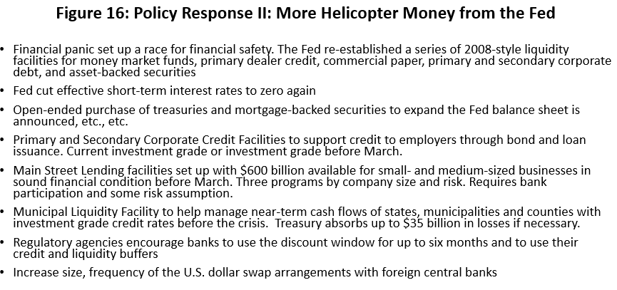
The Federal Reserve’s efforts are described in Figure 16. The Fed immediately pulled out the 2008-2009 Great Recession playbook, reopening emergency credit facilities, expanding its balance sheet, and cutting interest rates to zero. New or enhanced credit facilities are available for large corporations, small- and medium-sized businesses, and for states, municipalities, and counties. Depending on the specific facilities, risk is shared by the Treasury, participating financial institutions, and the Federal Reserve. Regulatory agencies have loosened regulations and lending requirements during the pandemic.

Is it A Recession? How Bad Is It?

On June 8, the National Bureau of Economic Research (NBER) announced that a U.S. recession had begun in February, marking the end of 128 months of continuous U.S. expansion. The NBER defines a recession as a “significant decline in economic activity spread across the economy, lasting more than a few months, normally visible in GDP, real income, employment, industrial production, and whole-sale-retail trade.”²¹ The committee recognized in making this statement that the pandemic and public health response resulted in a downturn with different characteristics than any prior recession.²²

The NBER does not consider government payments in its definition of recession because they do not contribute to production. However, in this Stay-Home Recession transfers must certainly be considered in terms of their likely economic effects and the depth of the downturn. Public health decisions initiated the recession and heavy federal stimulus is being used to offset its impact. After transfer payments are considered, the net economic impact of the downturn is substantially reduced by government transfers — although undoubtedly leaving a recession underway.

In previous versions of this report, I used the CBO’s severe pandemic/moderate downturn as the likely model for what we are seeing in this recession, reflecting the net difference between stay-home shock and the offsetting stimulus. After the long discussion above concerning the moderate economic effects of the 1918-19 pandemic, the workings of the CBO’s model of past pandemics, and the implications of the recent U.S. and Houston data, I come to a similar place as previous reports — with the CBO’s hypothetical severe pandemic/moderate recession serving as a useful model.

• It could be argued that the CBO severe pandemic is overkill with its 30 percent infection rate and 2.5 percent mortality rate. The current CDC May planning assumptions for hospitalizations and critical care call for a much lower mortality rate of 0.4 percent, although the COVID-19 infection rate may prove to be higher than 30 percent.
• The CBO recession never considered the huge up-front shock to the economy generated by public orders that were simultaneously imposed across every major metro area in the U.S. for six to eight weeks. This was not part of 2006 pandemic planning. But neither were the massive stimulus payments to offset public health orders.
• Also, the stay-home orders hit hard at virus-sensitive services sectors that employ the largest numbers of workers in the economy. These industries are not critical drivers of the economy, but in Houston for example, accommodation, entertainment, food and drink, health care, private education, and retail trade made up 1.1 million jobs or 33.2 percent of total payrolls.

We assume these plusses and minuses cancel out to approximate the CBO version of events as described earlier in Figures 3 and 4. This is a downturn in U.S. payroll employment of 3.0 percent beginning in the second quarter of this year, lasting four quarters, and then seeing a period of five quarters for employment to recover and return to the prior peak.

The measure that we use most often to follow the Houston economy is payroll employment, and the blue line in Figure 17 tracks the payroll downturn. It shows the effect of recession only, i.e., how the shrinking of the rest of the world affects Houston and makes its economic base smaller. Details are discussed later in the report, but the assumed combination of oil downturn and U.S. recession would cost Houston 72, 800 jobs as the worst of the recession arrives in 2020Q1. The revival of the U.S. economy through the rest 2021 is joined by an oil rebound in 2022 that results in all the local jobs lost to the virus restored by 2022Q2, with strong growth continuing through 2023.

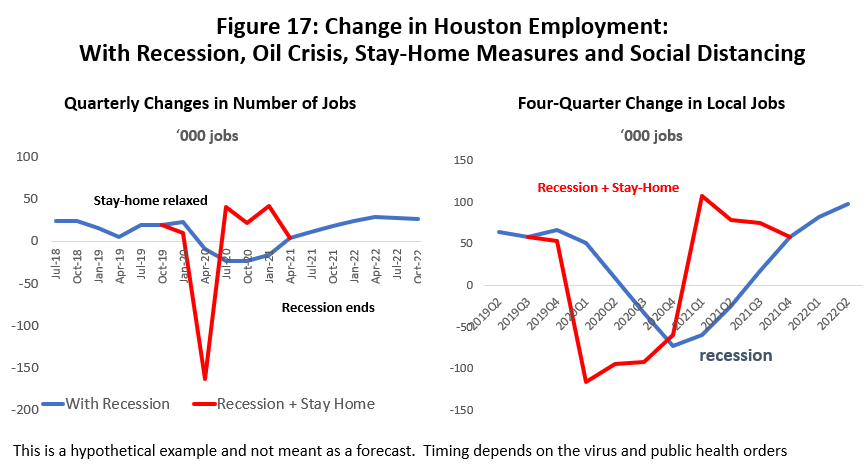
The red line in Figure 17 is the additional impact — on top of recession — of mandatory and reactive social distancing. These losses come mostly in small local businesses, and although they are non-basic, these sectors employ very large numbers of workers.

We simply have too little information to know how many of the job losses seen in March and April are the result of mandatory closings and how many are reactive distancing, but we should learn more about the division as the economy reopens. Meanwhile, I can only offer an illustrative example in Figure 17, with the red line showing how social distancing generates very large changes in the number of local jobs through 2020. First come large losses to the initial shock of stay-home orders and mandatory closings, then fewer losses and the return of some jobs as the economy struggles to reopen.

Figure 18 divides each month this year since March into a period of 10 days. The cells colored red are lock-down periods in Houston where enforced orders and reactive distancing results in the loss of 250,000 jobs. The yellow cells are partial re-opening stages or the re-imposition of partial orders as the virus worsens, with 150,000 jobs lost.²³

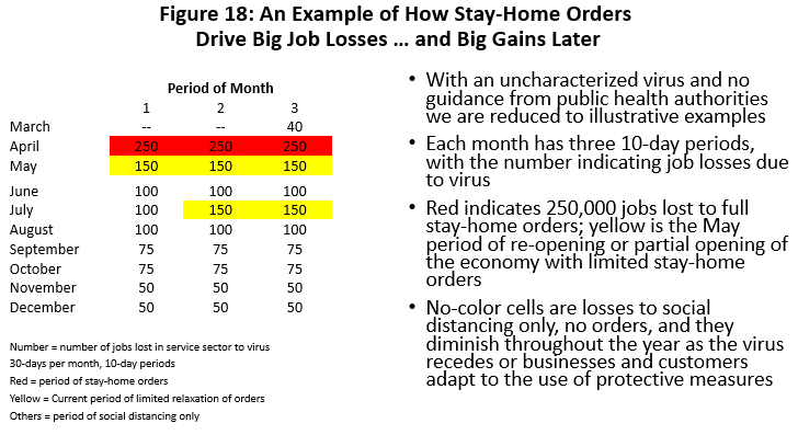
The cells with no color are reactive distancing only, and they assume that reactive distancing slowly disappears across the year as the virus recedes or as businesses and the public learn better ways to safely interact. Even with no orders in place, 100,000 jobs are lost to reactive distancing through August, slowly falling month after month to zero by early 2021.

Using this hypothetical illustration, by 2021Q1 the recession bottoms out, social distancing is no longer a problem, and the following five quarters see employment return to pre-virus levels. Houston’s job growth strengthens in 2021 as the U.S. recovery begins and turns even stronger in 2022 as rising energy prices allow oil to join the rebound.

Just as important, look at the swing in job growth from -163,200 jobs in 2020Q2 to a positive 40,600 in the following quarter. This is a perfectly plausible example of how these crazy swings in job growth stem from social distancing, and how they likely will continue through year-end. It is a hypothetical example, however, and should not be considered a projection or forecast in any sense whatsoever.²⁴

COVID-19 Wins Oil War: Cleaning Up the Mess

Recent events in world oil markets would make a fine soap opera with Houston’s oil sector as the protagonist, as large uncontrollable forces pushed it from one tragic turn of event to the next until an absolute bottom was reached with no apparent return in sight. This soap opera has had a few comic moments, but unfortunately, the overall entertainment value has been quite low for everyone concerned, whether they live in Houston or not.

• The current oil downturn began well before COVID-19, and originally centering on a 2019 credit crunch in the fracking industry. A legacy of cheap money, over-leverage, and poor management in many companies bred a wave of corporate delistings and bankruptcies. The rig count fell over 25% in 2019 and Houston lost 7,000 oil-related jobs before COVID-19 arrived in the U.S.
• The next turn of events was the brief Oil War, as two megalomaniacs briefly tried to prove that they could sell oil cheaper than the other. Would it be Russia or the Saudis who could withstand the pain of cheap oil for the longer time before the other buckled? The result in March and early April was a fleet of Saudi tankers flooding the world with oil and briefly driving the price of oil to single-digits.
• The Oil War that began in early March was short-lived, with COVID-19 declared an easy winner by mid-April, at least in terms of its ability to generate low oil prices. The shock from social distancing and stay-home orders dragged down economies around the world and led to a drop in oil demand that is variously estimated at 15 to 25 million barrels of oil per day. Suddenly, slowing the flow of too much oil into rapidly shrinking storage became a serious priority, and all hands were on deck as the U.S., Saudis, Russians, and the rest of OPEC+ sought to rapidly cut production. Even the chronic OPEC cheaters joined in cutting output through July.

The combination of lifting stay-home orders in many countries, combined with serious cuts in oil production, have resulted in early but significant progress in clearing up the huge overhang of oil that became apparent in April.

• The starting point for oil-market recovery is a return to market fundamentals with a price structure that is related to supply and demand. WTI and Brent crude have both stabilized at $35-$40 per barrel in recent weeks, faster progress than expected. The normal relationship between oil price and volatility has fallen into place for now, along with occasional signs of backwardation in futures markets (higher price today than tomorrow, indicating a current shortage). Inventories are drawing steadily for both crude and refined products.
• But it is not necessarily a straight path ahead. Solid OPEC+ compliance has been essential to the progress made thus far, but it is unlikely that current solidarity can last much past July. Cash-strapped U.S. producers are reopening shut-in capacity and will add 500,000 barrels of per day of production in July. Service companies in the Permian Basin are seeing fracking equipment return to work in July as producers seek to expand production with the completion of drilled-but-uncompleted wells.
• There is also uncertainty about the virus itself. Continued demand recovery is important to stability of oil prices. Texas and other sunbelt states are seeing a surge in COVID-19 that could set back U.S. reopening plans. China is seeing its own COVID surge in Beijing, a threat to what is now the world’s largest oil importer.
• Once market fundamentals are restored for oil, the fundamentals are not likely to be strong. Assuming that markets are working well by fall, most forecasts fall in the range of $40-$45 per barrel through much of 2021, with the optimists at only $50 and that arriving only in the second half of 2021.
• Our projection or planning assumptions for the rest of this year is $35-$40 per barrel, $40 until 2021Q3, $50 for the following two quarters, and the $60-$65 through 2026.

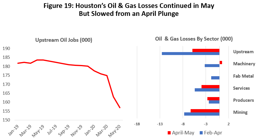
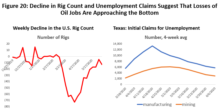
Oil-related employment in Houston shows a decline of 19,000 jobs since February and the beginning of the post-COVID period. Two-thirds of these losses came in March and April and continued at a slower pace in May. Figure 20 shows that the weekly declines in the U.S. rig count are now much smaller than before, and weekly claims for unemployment by Texas mining and manufacturing sectors are steadily falling back.²⁵

Our projected local oil-related job losses are only 24,500, requiring a return to relative stability over the second half of this year. Why so few jobs lost? After all, you see much bigger declines if you look back at 2015-16, with its loss of 77,300 upstream jobs. (See Figure 21)

But the bust of 2015-16 was a speculative downturn fed by several years of $100 oil, a period that saw Houston’s oil-related jobs shrink as fast as they had in the early stages of the 1980’s downturn. And only 18,700 of those oil jobs returned by mid-2019, when local oil employment began to shrink again in response to a credit crunch and another sharp drop in the rig count. By the time COVID-19 arrived, there were few oil-related speculative excesses left to wring out in Houston, and recent employment cuts have been to muscle and bone rather than fat.

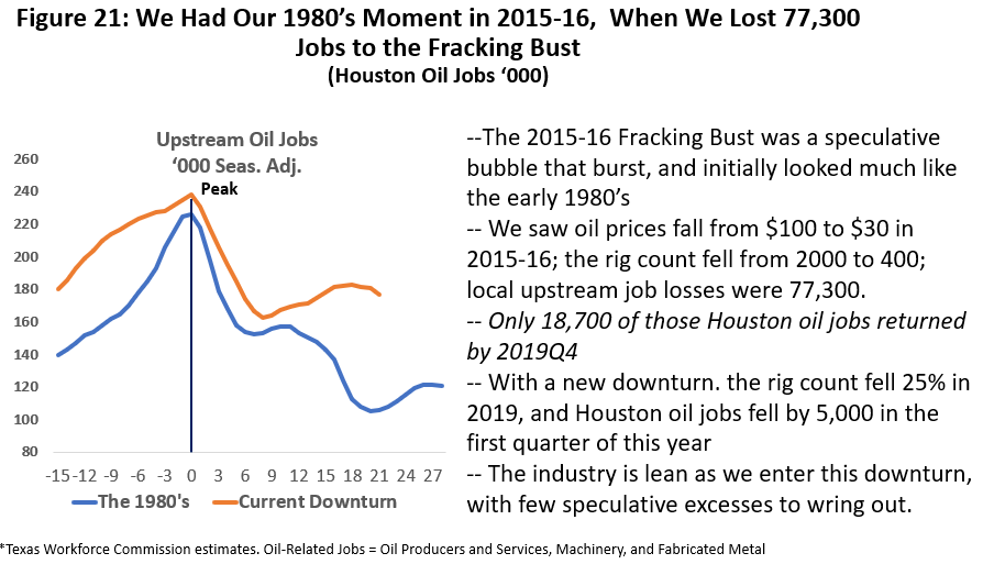
Figure 22 shows our estimates of the post-COVID rig count and the return of Houston’s oil-related jobs. While we might know something about where this number comes out in early 2021, the broken line for the rest of 2020 is not a number to be trusted, and a blank space might be a more appropriate representation.²⁶ As we stand in late June 2020, for example, the actual count of working rigs is below 300 rigs. By early- to mid-2021 we assume that oil-market fundamentals are back in place, and the continued solid line represents the basics and not the previous COVID-related and panic-driven shock.

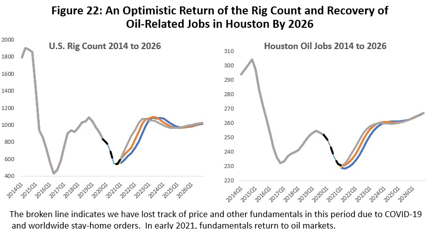
The assumptions about the recovery of rigs or oil employment in Figure 22 could look pessimistic compared to the boom of 2014, while many other readers will find this outlook extremely optimistic compared to 2019, especially if they see the fracking industry as permanently compromised by this downturn.

My own relative optimism is based on two roughly equivalent assumptions: (1) the world will again demand 100 million barrels of oil per day, i.e., the level of last February, and U.S. fracking and Canadian oil sands are necessary to make that happen, and (2) the price of oil will return to $55 to $65 per barrel or the long-run marginal cost of producing from those sources. Add to this that the oil-bearing rock is still there, the cost structure of getting the oil out of the rock is well understood, fracking has low barriers to entry in terms of scale of operation and capital needs, and the industry’s early success was among relatively small oil companies. In fact, it should be hard to stop this industry from returning once a successful management model is set.

The Global Outlook

The important news about the global economy is not that different from what we have seen across the U.S., including Houston. For every country, a poorly understood but dangerous virus is front and center, stay-home orders and business closings are widely implemented, a massive shock to the economy has briefly pushed every economic data series off a cliff, and there are early signs of reopening the economy. Where each country stands in the stay-home orders or reopening varies by when COVID-19 arrived there and the extent of local success in dealing with the virus.

China’s brush with COVID-19 came early and saw Q1/Q1 industrial output fall 8.4% early this year, while retail sales fell 19.0%, and GDP dropped 6.8%. Recent readings of Chinese economic data show the economy that is now expanding moderately and is expected to return to pre-COVID levels this year. A recent outbreak of COVID-19 in Beijing could put this at risk.

Measured the same way as China, Europe saw Q1 GDP fall 3.8%. But as Europe has reopened, the rate of contraction has slowed in Q2 according to its Purchasing Mangers’ Index. France, the second largest economy in Europe has seen its PMI move to slow expansion.

• Individual major European countries have issued fiscal packages that range from 1.4% to 4.5% of GDP; the European Central Bank has recently expanded its commitment to asset purchases to 1.35 trillion euros.
• After the apparent failure of the European Union to authorize 540 billion euros in so-called coronabonds as joint fiscal policy to respond to the crisis, a more ambitious Stabilization Fund proposal has come forward to launch a huge redistribution of virus relief to Europe’s poorest countries. It would be 750 billion euros in grants and loans, with $500 billion in lending under very long maturity bonds. The fiscal split between northern and southern countries remains a barrier to completing the deal.
• Before COVID-19, Europe had never cleaned up its banking system after the 2008-09 crisis. Italy is a possible flash point. It holds the third-largest sovereign debt in the world, now at 155% of its GDP, while the economy is expected to shrink 7-8 percent this year. Much of Italian debt is held by French and German banks.

Japan is another economy that was struggling before COVID-19 and continues to do so. The second quarter will likely mark its third consecutive decline in GDP. Total stimulus is now $2.2 trillion, with $1 trillion just added in June as payments to individuals and small and medium business.

Emerging markets are seeing rapidly rising COVID-19 cases in India, Russia, Brazil, and a number of other Latin American countries. This simply adds to expectations of a very uneven global recovery.

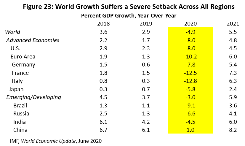
The bottom line for the global outlook is an IMF forecast for global growth is a 4.9 percent decline in GDP this year, with a sharp rebound of 5.5 percent in 2021. (See Figure 22) While the recession has quickly fallen into place, the extent and timing of recovery present considerable risk.

Summary and Conclusions on the Economy

We have all the basics in hand from the analysis above. Recall that much of our discussion concerning 2020 and early 2021 is based on plausible illustrative examples and cannot be called a meaningful forecast or prediction. The structural break in the economy created by COVID-19 prevents us from understanding very well where we are right now, much less where we are going in the future. The near-term value of statistical models is low to nonexistent. Only as we move into next year, as economic fundamentals begin to matter again, can we have a better sense of the direction of the local economy.

How do we pull all our assumptions and examples together for Houston’s near-term outlook? The outline of events runs as follows.

• A U.S./Houston recession begins in 2020Q2, finds a trough in 2021Q1, and recovers lost payroll jobs by 2022Q2.
• Oil prices fall to roughly $40 per barrel for seven quarters from 2020Q1 to 2021Q3.
• A double recovery comes as recession ends in 2021Q2 and oil price returns to $60-$65 in 2022Q3. The deeper and longer the downturn, the faster and longer the recovery. A dismal 2020 and early 2021 are followed by two years of strong growth.

The Important assumptions?

• For the short-run — quarterly results through at least early next year – neither markets nor economic models are working. By the first quarter of next year, we should be able to have some faith in our understanding of economic outcomes, but even that depends on little understood progress in containing the virus.
• We are assuming that monetary and fiscal policy can effectively fill the stay-home and social distancing employment gap left by COVID-19. The huge employment losses in early 2020 will be substantially offset by income from the stimulus. We assume stimulus is provided to the extent to support a continued viral outbreak.
• There is no permanent damage to the American oil industry due to the long period of oil prices at or below $40 per barrel.
• Houston’s economy returns to its long-run annual growth rate for payroll employment growth near 2.1 percent. The period of growth lost to the COVID-19 recession is not recovered, however.

The net change in the number of payroll jobs in Houston from 2020-2026 is shown in Figure 22. The chart on the left is the number of jobs measured from fourth quarter to fourth quarter, and on the right are the year-over-year changes. Both charts show the change in total payrolls, including specific contributions from both the U.S. business cycle and local social distancing. The social distancing figure uses the hypothetical example in Figure 18.

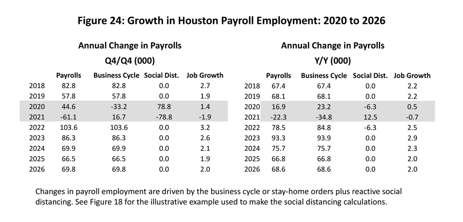
This downturn in the economy extends from 2020Q2 to 2021Q1, cutting across the two calendar years. Measured from peak to trough there are 72,000 jobs lost, with 2021Q2 marking the first quarter of recovery from recession. As expected, strong growth follows that and is driven first by U.S. economic expansion in 2021, followed by higher oil prices in 2022. By 2024, Houston’s long-run growth path for payrolls has returned to near 2.1 percent or its long-run average since 1990.

Our analysis is meant to be illustrative but tries to trace a realistic future once a series of initial assumptions are made. There is value, for example in understanding how social distancing drives the huge and frightening swings in employment we have seen this year, and how the stimulus payments largely offset these early job losses with income gains. But at the heart of all the calculations is the unknown course of COVID-19 and the reaction of public health officials as the virus spreads. We have built the economic analysis around assumptions about length of the downturn and its depth that are based on the behavior of the virus, for example, but with few solid epidemiological facts that support those assumptions. It remains a largely unknown and highly uncertain economic future until the virus is somehow tamed by treatment, vaccine or herd immunity.

Written by Robert W. Gilmer, Ph.D.
C. T. Bauer College of Business/Institute for Regional Forecasting
June 28, 2020

---

¹ The previous reports were R.W. Gilmer, “Houston’s Economic Outlook Reshaped by COVID-19 and the Oil Price War,” Institute for Regional Forecasting, University of Houston, March 22,2020 and “Houston’s Economic Outlook Reshaped by COVID-19 and the Oil Price War: An Update and Extension,” IRF, April 8, 2020.

² Thomas A. Garrett, “Pandemic Economics: The 1918 Influenza and Its Modern Day Implications,” Economic Review, Federal Reserve Bank of St. Louis, 90(2) March/April 2008, pp. 77.

³ Centers for Disease Control and Prevention, COVID-19 Pandemic Planning Scenarios, May 2020.

⁴ Congressional Budget Office, “A Potential Influenza Pandemic: Possible Macroeconomic Effects and Policy Issues,” revised July 27, 2006. This CDC report explicitly uses the 1957-58 recession as a model for the economic consequences of a mild pandemic. It is discussed at length later in the report.

⁵ Robert J. Barro, and Jose F. Ursúa (2008). "Macroeconomic Crises since 1870." Brookings Papers on Economic Activity, 39 (Spring): 255-350

⁶ Studies that are widely cited but likely suffering from specification error or serious data issues are Sergio Correia, Stephan Luck, and Emil Verner, “Pandemics Depress the Economy, Public Health Interventions Do Not: Evidence from the 1918 Flu,” SSRN Discussion Paper 3561650, revised April 10, 2020 and Elizabeth Brainerd and Mark V. Siegler, “The Economic Effects of the 1919 Influenza Epidemic,” London: Centre for Economic Policy Response, Discussion Paper No. 3791 who both ignore WW1 mortality and effectively merge two recessions, and Thomas A. Garrett, “War and Pestilence as Labor Market Shocks: U.S. Manufacturing Growth 1914 to 1919,” Working Paper Series, 2006018C, Federal Reserve Bank of St. Louis, Revised October 2007.

⁷Wesley C. Mitchell and Arthur F. Burns, Measuring Business Cycles, New York: National Bureau of Economic Research, 1946.

⁸ Francois R. Velde, “What Happened to the U.S. Economy During the 1918-19 Influenza Epidemic? A View Through High-Frequency Data,” Chicago: Federal Reserve Bank of Chicago, Working Paper 2020-11, Revised April 17, 2020.

⁹ Robert J. Barro, Jose F. Ursúa, and Joanna Weng, , “The Coronavirus and the Great Influenza Pandemic: Lessons from the “Spanish Flu” for the Potential Effects on Mortality and Economic Activity,” NBER Working Paper 26866, Revised April 2020.

¹⁰ Federal Reserve Bank of Philadelphia, Survey of Professional Forecasters, Second Quarter, May 15, 2020.

¹¹ The depth and timing of decline and recovery of a typical U.S. recession since 1948 is easy to mimic. However, for the mild case with its significant slowdown in GDP that does not turn into recession, we assumed a growth recession, i.e., a period that sees GDP slow sufficiently to cause employment to decline.

¹² Howard Markle, et al., “Nonpharmaceutical Interventions Implemented by U.S. Cities During the 1918-1919 Influenza Epidemic,” Journal of the American Medical Association, vol. 298, #6, August 8, 2007, pp. 644-54

¹³ Martin C. Bootsma and Neil M. Ferguson, “The Effectiveness of Public Health Measures on the 1918 Influenza Epidemic in U.S. Cities,” Proceedings of the National Academy of Sciences, vol. 104, no. 18, May 1, 2007, pp. 7588-7593.

¹⁴ Richard J. Hatchett, Carter E. Mecher, and Mark Lipsitch, “Public Health Interventions and Epidemic Intensity During the 1918 Influenza Epidemic,” Proceedings of the National Academy of Sciences, vol. 104, no. 18, May 1, 2007, pp. 7582-7587.

¹⁵ About 75 percent of Americans have sick leave that would have covered this time away from work if it played out like past pandemics. This would have reduced the current public burden of unemployment as private employers would have borne much of the cost of time away from work.

¹⁶ The problem is that the stay-home orders simultaneously generated severe economic shock (part virus and part public orders) and huge job losses (part mandatory orders and part reactive social distancing). We also need to better understand which part of the social distancing losses to attribute to reactive behavior and how much was mandatory. We will only get a glimpse into this once all public orders are lifted.

¹⁷ Economists will tell you that there is a trade-off between the number of lives lost and the economy. It is a decision made all the time, most obviously with health and safety regulations. It is impossible to impose safety standards that would drive the number of deaths to zero without halting economic activity, and the question becomes how many lives should be lost to allow economic progress to continue and at what rate. It is a problem not discussed nearly enough in the current pandemic.

¹⁸ Houston’s economic base contains upstream oil (producers, services, machinery, and fabricated metals) and downstream oil (refining, chemicals, and plastics). There are also pipelines, non-oil manufacturing, and selected sectors in construction, professional and business services, wholesale trade and air transportation. Calculations use location quotients for excess employment as drawn from a typical textbook. Also see Scott J. Brown, N. Edward Coulson, and Robert F. Engle, “On the Determination of the Regional Base and Regional Multipliers,” Regional Science and Urban Economics,” (1992), vol. 22, pp. 619-635.

¹⁹ Houston’s Purchasing Managers’ Index (PMI) has been produced monthly by the local chapter of the Institute for Supply Management since 1997. Their calculation of Houston’s index includes seven variables, four of which overlap with the national index. The Houston index has two inventory measures (final goods and goods in process) while the national index combines both final goods and in-process inventory into one variable. To better mimic the national index more closely, I compute the Houston index by using the common four variables from the national index and add final goods inventory. Like the national index, my version has all five variables combined by weighting equally. The final index is then seasonally adjusted. The break-even point between expansion and contraction is 50 for both indexes.

²⁰ The average American working on a payroll earned $936 per week in 2019 or $48,672 in wages or salary. This excludes benefits.

²¹ The NBER’s Recession Dating Procedure is found here: https://www.nber.org/cycles/jan08bcdc_memo.html#:~:text=A%20recession%20is%20a%20significant,%2C%20and%20wholesale%2Dretail%20sales.

²² For the NBER determination of the February 2020 peak in U.S. Economic Activity and the announcement of a new recession, see https://www.nber.org/cycles/june2020.html

²³ As this is written, Houston is seeing a surge in COVID-19 cases associated with the reopening of the Texas economy that is perhaps capable of threatening the threshold requirement for critical care capacity. As the surge continued into July, it has become necessary to re-impose restrictions like closing bars and limiting restaurant capacity more stringently (the yellow cells). If the outbreak turns worse, it could stringent stay-home restrictions and nonessential business closings. (red cells).

²⁴ Also remember that the blue line is a hypothetical Congressional Budget scenario. We are assuming that something like the CBO’s “severe pandemic” underlies an on-going U.S. recession. So, we have in Figure 18 a plausible fiction about the U.S. recession added to a hypothetical example about social distancing.

²⁵ The steady declines continued through the first two weeks of June.

²⁶ The forecast uses a dummy variable for 2020Q2 to remove the “non-economic/COVID-driven” decline in the rig count or local oil jobs, then forecasts by using the smaller decline in the “economic” component only, i.e., assuming the economy continued to respond to basic fundamentals. Assuming economic rules are restored by early 2021, perhaps we will be back on a realistic economic track by that time.